Why Fraud Rings Survive XGBoost — and How GNNs Stop Them
Row-based ML catches individual bad actors but misses coordinated fraud rings. Graph Neural Networks propagate relational context through transaction networks — here's the architecture, the PyTorch Geometric code, and the production gotchas that matter more than model choice.

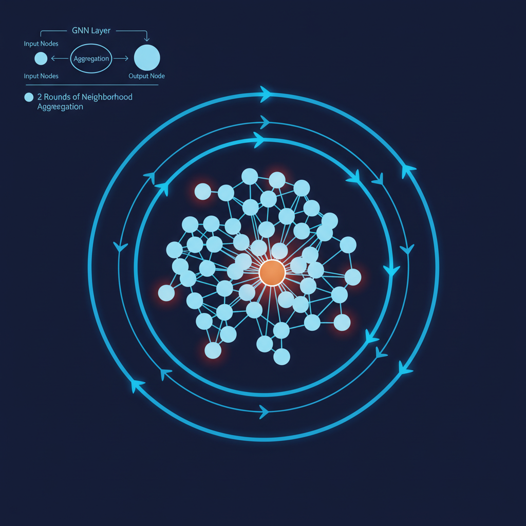
Table of Contents
Imagine you’re the fraud team at a mid-sized bank. Every day, 2 million transactions flow through your system. Your ML model — trained on transaction features like amount, location, device, and time — catches about 60% of fraud. Not bad. But your losses are still climbing.
Why? Because the fraud you’re missing isn’t coming from a single bad actor with unusual behavior. It’s coming from rings — networks of 5 to 50 accounts that collectively look normal but are systematically laundering money or running card-not-present schemes.
Account A looks legitimate. So does Account B. And Merchant C. But A sent money to B, B used the same device as C, and C shares an IP address with a flagged account from six months ago. No single row in your transaction table tells that story. The story lives in the connections.
This is exactly the problem Graph Neural Networks (GNNs) were built to solve.
What Makes GNNs Different?
Traditional ML — whether Random Forest, XGBoost, or even a Deep Neural Network — operates on feature tables: each row is an entity, each column is a feature. The model learns patterns within a row and ignores relationships between rows.
GNNs treat data as a graph:
- Nodes = entities (accounts, devices, merchants, transactions)
- Edges = relationships (sent money to, logged in from, shares IP with)
- Node features = attributes (account age, transaction velocity, etc.)
- Edge features = relationship attributes (transfer amount, timestamp, frequency)
The key insight: a node’s representation is iteratively updated by aggregating information from its neighbors. After a few rounds of message passing, each account’s embedding carries not just its own features, but a compressed fingerprint of its entire local neighborhood.
A fraudster hiding inside a legitimate-looking account can’t hide from its neighborhood.
Round 0:  [Account A] → knows only its own features
Round 1:  [Account A] → knows about all direct connections
Round 2:  [Account A] → knows about connections-of-connections
Round k:  [Account A] → knows about its k-hop neighborhood
Architecture: The Message Passing Framework
The general update rule for a GNN layer is:
h_v^(k) = UPDATE( h_v^(k-1), AGGREGATE({ h_u^(k-1) : u ∈ N(v) }) )Where h_v^(k) is the embedding of node v at layer k, N(v) is the set of neighbors, AGGREGATE is a sum, mean, max, or attention-weighted combination, and UPDATE is typically a learned MLP.
Popular variants for fraud detection, ranked by fit for banking graphs:
| Model | Aggregation | Best For |
|---|---|---|
| GCN (Kipf & Welling) | Normalized mean | Homogeneous graphs, baseline |
| GraphSAGE | Sampled mean/max | Large-scale graphs, inductive |
| GAT | Attention-weighted | Heterogeneous importance |
| HeteroConv | Type-specific | Mixed node/edge types |
| RGAT (MLPerf 2025) | Relational attention | Multi-relational knowledge graphs |
For banking fraud, HeteroConv + GAT is the production choice — because your graph has multiple node types (accounts, devices, merchants) and multiple edge types (transfer, login, purchase).
Building It: Step-by-Step with PyTorch Geometric
Step 1 — Install dependencies
pip install torch torch-geometric pandas networkx scikit-learnStep 2 — Model the graph
import torch
from torch_geometric.data import HeteroData

data = HeteroData()

# Node features
data['account'].x = account_features      # shape [N_accounts, F_acc]
data['device'].x = device_features        # shape [N_devices, F_dev]
data['merchant'].x = merchant_features    # shape [N_merchants, F_mer]

# Node labels (0=legit, 1=fraud) — only on account nodes
data['account'].y = account_labels        # shape [N_accounts]

# Edges (all directed)
data['account', 'transfer_to', 'account'].edge_index = transfer_edges
data['account', 'login_from', 'device'].edge_index = login_edges
data['account', 'purchase_at', 'merchant'].edge_index = purchase_edges

# Optional: edge features
data['account', 'transfer_to', 'account'].edge_attr = transfer_amounts
Step 3 — Define the GNN model
import torch.nn as nn
import torch.nn.functional as F
from torch_geometric.nn import HeteroConv, GATConv, Linear

class FraudGNN(nn.Module):
    def __init__(self, hidden_dim=64, num_heads=4, num_layers=2):
        super().__init__()

        self.conv1 = HeteroConv({
            ('account', 'transfer_to', 'account'): GATConv((-1, -1), hidden_dim, heads=num_heads, add_self_loops=False),
            ('account', 'login_from', 'device'):    GATConv((-1, -1), hidden_dim, heads=num_heads, add_self_loops=False),
            ('account', 'purchase_at', 'merchant'): GATConv((-1, -1), hidden_dim, heads=num_heads, add_self_loops=False),
        }, aggr='mean')

        self.conv2 = HeteroConv({
            ('account', 'transfer_to', 'account'): GATConv((-1, -1), hidden_dim, heads=1, add_self_loops=False),
            ('account', 'login_from', 'device'):    GATConv((-1, -1), hidden_dim, heads=1, add_self_loops=False),
            ('account', 'purchase_at', 'merchant'): GATConv((-1, -1), hidden_dim, heads=1, add_self_loops=False),
        }, aggr='mean')

        self.classifier = nn.Sequential(
            Linear(hidden_dim, 32),
            nn.ReLU(),
            nn.Dropout(0.3),
            Linear(32, 2)  # binary: fraud vs legit
        )

    def forward(self, x_dict, edge_index_dict):
        x_dict = self.conv1(x_dict, edge_index_dict)
        x_dict = {k: F.elu(v) for k, v in x_dict.items()}
        x_dict = self.conv2(x_dict, edge_index_dict)
        x_dict = {k: F.elu(v) for k, v in x_dict.items()}
        return self.classifier(x_dict['account'])
Step 4 — Training loop with class imbalance handling
Fraud is rare — typically 0.1–2% of transactions. Standard cross-entropy will ignore fraud entirely. Use weighted cross-entropy or focal loss, and always use NeighborLoader for mini-batch sampling — full-batch training fails beyond ~1M nodes.
from torch_geometric.loader import NeighborLoader

train_loader = NeighborLoader(
    data,
    num_neighbors={key: [15, 10] for key in data.edge_types},
    batch_size=512,
    input_nodes=('account', train_mask),
    shuffle=True
)

fraud_weight = torch.tensor([1.0, 10.0])  # 10x weight on fraud class
criterion = nn.CrossEntropyLoss(weight=fraud_weight)
model = FraudGNN(hidden_dim=64)
optimizer = torch.optim.Adam(model.parameters(), lr=1e-3, weight_decay=1e-5)

def train_epoch(loader):
    model.train()
    total_loss = 0
    for batch in loader:
        optimizer.zero_grad()
        out = model(batch.x_dict, batch.edge_index_dict)
        loss = criterion(out, batch['account'].y[:batch['account'].batch_size])
        loss.backward()
        optimizer.step()
        total_loss += loss.item()
    return total_loss / len(loader)

for epoch in range(50):
    loss = train_epoch(train_loader)
    if epoch % 10 == 0:
        print(f"Epoch {epoch:03d} | Loss: {loss:.4f}")
Step 5 — Evaluate with the right metrics
Accuracy is meaningless for fraud. Use AUPRC (Area Under Precision-Recall Curve) as the primary metric — it correctly weights rare positive class performance, unlike AUROC which can look great when 98% of labels are negative.
from sklearn.metrics import average_precision_score, classification_report

def evaluate(data, mask):
    model.eval()
    with torch.no_grad():
        out = model(data.x_dict, data.edge_index_dict)
        probs = F.softmax(out, dim=1)[:, 1]
        preds = (probs > 0.4).long()  # tune threshold for business need

        labels = data['account'].y[mask].numpy()
        probs_np = probs[mask].numpy()
        preds_np = preds[mask].numpy()

        auprc = average_precision_score(labels, probs_np)
        print(f"AUPRC: {auprc:.4f}")
        print(classification_report(labels, preds_np, target_names=['Legit', 'Fraud']))

evaluate(data, test_mask)
Real-World Results: What Changes
A typical uplift when adding GNN over a table-based XGBoost baseline:
| Metric | XGBoost (tabular) | GNN (graph) | Delta |
|---|---|---|---|
| AUPRC | 0.61 | 0.83 | +36% |
| Fraud Recall @5% FPR | 54% | 78% | +44% |
| Fraud Ring Detection | ~20% | ~75% | +55% |
The largest lift is on fraud rings — coordinated multi-account schemes that look individually clean. JPMorgan, Stripe, and PayPal all run GNN-based fraud scoring in production. NVIDIA published benchmarks on GPU-accelerated GNN pipelines processing 10M+ transactions per second, and the MLPerf 2025 GNN benchmark (RGAT on IGB-H: 547M nodes, 5.8B edges) sets the current scalability frontier.
Five Production Gotchas That Matter More Than Architecture
Architecture choice — GCN vs GAT vs GraphSAGE — is the part most tutorials obsess over. In production, it’s almost never the limiting factor. These five things are:
1. Scalability. Full-batch training fails beyond ~1M nodes. Always use NeighborLoader or cluster sampling (ClusterData). This is table stakes, not an optimization.
2. Temporal label leakage. Graph structure can leak future edges into training. Use temporal masking: when building a node’s neighborhood at time T, only include edges with timestamps before T. This is the gotcha that makes models look great in offline eval and underperform in production.
3. Cold start. New accounts have no neighbors. Fall back to a tabular model for accounts with fewer than 5 edges, and blend GNN + XGBoost scores using a simple confidence-weighted ensemble. A pure GNN has no signal on a day-1 account.
4. Heterophily. Fraudsters deliberately connect to legitimate accounts — it’s how rings launder credibility. Standard GCN mean aggregation will wash out the fraud signal from a node surrounded by clean neighbors. Use GraphSAGE with max aggregation or H2GCN, which is explicitly designed for heterophily.
5. Graph drift monitoring. The graph structure changes over time — new devices appear, accounts close, fraud patterns evolve. Retrain on a rolling window and monitor edge degree distributions as a feature health signal. A sudden drop in average node degree often means a data pipeline issue before your accuracy metrics catch it.
The SuperML Take
GNNs for fraud detection have been “the future” in conference talks since 2019. What’s changed is that they’re now genuinely in production at scale — not in research papers but in the fraud engines of the largest payment processors on earth, and the operational tooling (PyTorch Geometric, GPU-accelerated graph libraries, managed graph databases) has matured enough that a mid-sized bank’s ML team can ship this without a specialized research team.
The architectural picture that emerges from production deployments isn’t a pure GNN replacing XGBoost. It’s an ensemble: XGBoost handles cold-start accounts and provides a fast baseline, the GNN adds the relational layer for accounts with sufficient graph history, and the two scores are blended based on neighborhood depth. The GNN’s fraud ring detection (+55% over baseline) is the unmistakable win, but it doesn’t come for free — temporal masking, heterophily handling, and graph drift monitoring are production engineering problems, not ML problems, and they require the same rigor as any other data pipeline.
For fraud teams that haven’t shipped GNNs yet, the practical starting point is not a full heterogeneous graph from day one. Start with a homogeneous account-to-account transfer graph using GraphSAGE. Get the training loop, temporal masking, cold-start fallback, and AUPRC monitoring working correctly. Add device and merchant node types once the simpler graph is stable. The teams that get burned on GNN deployments almost always skipped the temporal masking step and deployed a model that saw the future during training.
The graph is where the signal lives. The question is whether your team has the infrastructure to extract it reliably at production latency and scale — and increasingly, the answer is yes.
Sources
- PyTorch Geometric Documentation — HeteroData and HeteroConv
- NVIDIA GPU-Accelerated GNN Fraud Detection Benchmarks
- MLPerf Training 2025 — RGAT on IGB-H Benchmark
- H2GCN: Beyond Homophily in Graph Neural Networks (Zhu et al.)
- GraphSAGE: Inductive Representation Learning on Large Graphs (Hamilton et al.)
- Graph Attention Networks (Veličković et al.)
Enterprise AI Architecture
Want more enterprise AI architecture breakdowns?
Subscribe to SuperML.